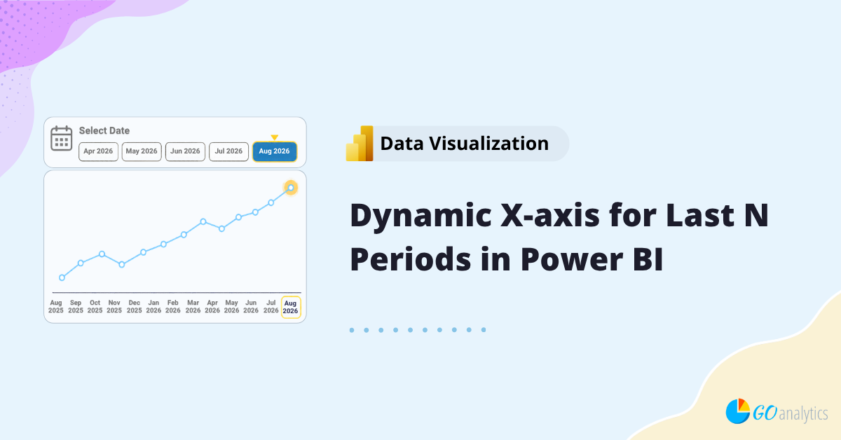
In this blog post, we walk you through how to create a dynamic x-axis for the last N date periods in a Power BI timeseries chart.
Date filters and slicers are useful for letting users choose which period they want to analyze. But sometimes selecting a date should do more than simply filter a visual for that period. Sometimes, we want to put that specific period into context by showing the last N periods.
For example, suppose a user selects August 2026. Instead of displaying only August 2026, we may want a line chart to display the previous 12 months ending in August 2026. And let’s say we want this to be dynamic based on a date filter selection.
Let’s tackle it together using an example with Canadian Gross Domestic Product (GDP) data.
The Problem with a Standard Date Slicer
Suppose we have a report page with a line chart showing GDP by month and year and a slicer visual using a Month & Year column from our Dates table. If a user selects August 2026, the expected Power BI behavior is straightforward: the slicer filters the Dates table to August 2026, and the chart displays only that month.
That’s technically correct, but it is not what we want.
We want the selected date to act as the endpoint of our visual so that if we choose August 2026, and our window is the last 12 months, then the chart should display the 12-month period ending in August 2026 (i.e., the X-axis of the chart should show us August 2025 through to August 2026).
⚠️ Note: Power BI offers several ways to filter report data, including slicers and the Filter pane. To learn more about these differences, check out our guide on using slicers vs. the Filters pane in Power BI.
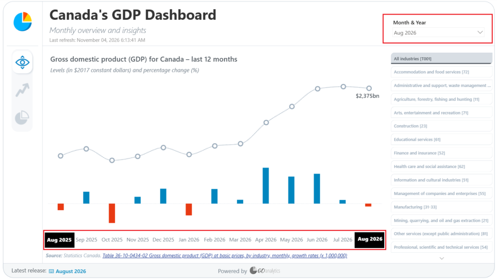
To accomplish this, we need to separate the date used to filter our report from the date used to display values on the X-axis.
How do we do that?
Step 1: Create a Second Dates Table
The first step is to create a second date table. In our example, we’ll call it Dates to Display.
This table contains the same dates as our primary Dates table, but it serves a different purpose. Our regular Dates table continues to control the slicer, while Dates to Display controls which periods appear along the X-axis. In our example, we simply create a duplicate of our Dates table.
In the data model, create a many-to-one relationship from the original Dates table and Dates to Display table on the Date column of each table; make cross-filtering a single direction.
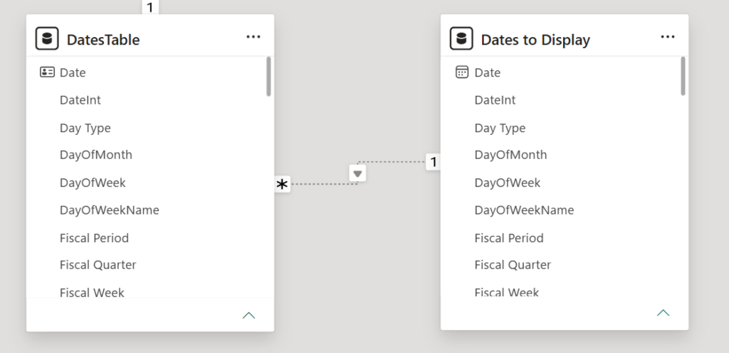
The inactive relationship is intentional. We don’t want the second date table automatically filtering the primary date table. Instead, we’ll activate that relationship only when our calculation needs it using the USERELATIONSHIP function.
The USERELATIONSHIP function allows a DAX calculation to use an existing relationship for the duration of that calculation, including an inactive relationship.
Step 2: Define the Periods to Display
Next, we need a measure that determines the date range we want to display (note: this measure uses our root measure of [Real GDP], which was calculated previously).
The basic logic is:
- Find the date period selected by the user
- Calculate the previous N periods from that date
- Remove the slicer’s direct date filter from the calculation
- Calculate the result using the dates appearing on the X-axis
Let’s break it down.
One of the key functions to enable the magic here is DATESINPERIOD.
The DATESINPERIOD function returns a set of dates based on a starting date, a number of intervals, and an interval type such as month, quarter, or year. A negative interval moves backward from the starting date, making it useful for rolling-period calculations.
Note that a positive interval moves forward so it could be useful for showing forecasts (i.e., current period and next 12 months forecast).
For steps 1 and 2 above, here is the DAX code we’ll need:
Real GDP (Last 12M) =

VAR SelectedDate =
    MAX ( 'Dates'[Date] )

VAR PeriodToDisplay =
    DATESINPERIOD (
        'Dates'[Date],
        SelectedDate,
        -12,
        MONTH
    )
In the DAX code above, we are creating two variables. The SelectedDate variable captures the end of the period selected in the report, while PeriodToDisplay creates the historical date window.
Microsoft specifically documents DATESINPERIOD as a table function designed to be passed as a filter to CALCULATE for standard date intervals such as days, months, quarters, and years.
If you’re looking to calculate a rolling average rather than dynamically change the periods displayed on a visual, check out our guide to rolling average measures in Power BI.
For steps 3 and 4, we continue with our DAX measure below:
RETURN
CALCULATE(
    [Real GDP],
    REMOVEFILTERS( 'Dates' ),
    KEEPFILTERS( PeriodToDisplay ),
    USERELATIONSHIP( 'Dates'[Date], 'Dates to Display'[Date] )
)
The full measure then uses functions such as CALCULATE to adjust the filter context of our measure, REMOVEFILTERS to remove the filters from our original Dates table, KEEPFILTERS to apply the last 12-month period filter context, and USERELATIONSHIP to call upon our inactive relationship. This DAX allows our measure then to evaluate the underlying measure (i.e., Real GDP in our example) over the appropriate dates.
In its entirety, this is our new measure that we will place on our visual:
Real GDP (Last 12M) =

VAR SelectedDate =
    MAX ( 'Dates'[Date] )

VAR PeriodToDisplay =
    DATESINPERIOD (
        'Dates'[Date],
        SelectedDate,
        -12,
        MONTH
    )

RETURN
CALCULATE(
    [Real GDP],
    REMOVEFILTERS( 'Dates' ),
    KEEPFILTERS( PeriodToDisplay ),
    USERELATIONSHIP( 'Dates'[Date], 'Dates to Display'[Date] )
)
Step 3: Configure the X-axis
The final piece is configuring the visual.
Instead of placing the Month & Year column from the primary Dates table on the X-axis, use the equivalent field from Dates to Display.
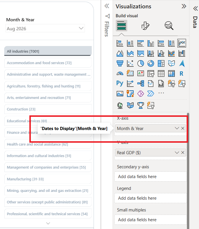
This is what separates the two jobs:
- Dates controls the user’s date selection
- Dates to Display controls the dates shown on the X-axis
- DAX determines the window of dates that should return values
Now, when the user changes the selected period, the endpoint of the chart changes with it while retaining the historical periods leading up to that date.
Use the Same Pattern for Different Period Ranges
Although our example uses the previous 12 months, you can use the same pattern for any date period range you would like.
For example, you could create:
- Previous 3 months
- Previous 6 months
- Previous 18 months
- Previous 8 quarters
- Previous 5 years
- Next 12 months
The DATESINPERIOD function currently supports day, month, quarter, and year intervals when using a date-column input, so the same general approach can be adapted to different reporting requirements.
You can also reverse the concept to display periods after a selected date, which can be useful when displaying forecasts or other forward-looking values.
Wrapping It Up...
The main idea behind this technique is fairly simple: the date selected by the user doesn’t have to be the only date displayed on the visual. By separating the report’s date selection from the dates used on the X-axis, you can use the selected period as an endpoint and dynamically display the N periods leading up to it. Using the provided DAX example, you can adjust the period range to suit the business questions your userbase would like to answer.
Need Help Getting Started With Power BI?
Our Microsoft Certified consultants can help with the implementation of Power BI in your organization