
In this blog post, we provide a practical guide to creating rolling average (i.e., last 30 days) measures in Power BI using the built-in DAX (Data Analysis Expressions) programming language.
A rolling average (also called a moving average) smooths out short‑term fluctuations so you can see the underlying trend more clearly. Instead of looking at just today’s value, a rolling average looks at the average over the last N days/weeks/months.
Typical use cases in Power BI:
- Sales trends (7‑day or 30‑day rolling average revenue)
- Website traffic (rolling average sessions to smooth weekend dips)
- Operational metrics (rolling average tickets created, units produced, etc.)
- Stock price trends (50-day and 200-day moving averages)
The problem that rolling averages solve is that without them, our line charts can be noisy and misleading (for example, big spikes from promotions or month‑end pushes). With rolling averages, decision makers see direction and momentum, which leads to better questions and better decisions.
To better understand this concept, let’s do it together! We’ll take our last example and analyze Microsoft’s (MSFT ) stock price.
Prerequisites: Date Table & Model Setup
Before writing DAX, let’s make sure our model is ready. Rolling averages rely heavily on a proper Dates table.
Here’s what we need:
- A Dates table with at least a ‘Dates’[Date] column with one row per day, no gaps
- A year (‘Dates’[Year]), month (‘Dates’[Month]), month number (‘Dates’[Month Number]) dimensions for visualizations
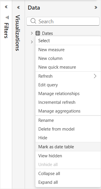
Once our Dates table is ready, let’s go ahead and mark it as a Date table in Power BI. We can do this by navigating to the Data pane in Power BI Desktop, clicking the ellipsis (…) next to our Dates table, and selecting Mark as date table.
Next, we need to set up our data model. Let’s be sure we have a relationship from our Dates table to our fact table’s (the MSFT stock prices) date column.
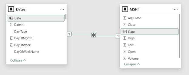
⚠️ Power BI’s time intelligence functions require a proper Date table. In the absence of this table, all time-intelligence functions (DATESINPERIOD, DATEADD, etc.) will give inconsistent results.
Step 1: Create Base Measure
All rolling measures should be built on top of a base measure, not a raw column. This keeps your model clean and reusable. For our example, our base measure is the Average Closing Price:
Average Closing Price = AVERAGE ( MSFT[Close ] )Note that this measure respects all existing filters (i.e., date).
Step 2: Rolling Sum vs Rolling Average
Our example above is somewhat of an edge case. Most of the time you will be dealing with a base measure that is summing a column (i.e., Total Sales = SUM ( Sales[Amount] )).
In the case of a base measure that is already calculating the average, we can be finished with just one step. However, when we have a sum analysts often start by jumping straight into a rolling average and get tangled up in the math. It’s often easier to first create the rolling sum (i.e., total sales over last 90 days) and then convert it to an average by dividing by the number of periods.
Step 3: Rolling Average DAX
Returning to our example, our DAX measure then follows:
50-Day Moving Average =
CALCULATE (
    [Average Closing Price],
    DATESINPERIOD (
        'Dates'[Date],
        MAX ( 'Dates'[Date] ),  -- anchor date in current filter context
        -50,                    -- go back 30 days
        DAY
    )
)
What this does:
- MAX(‘Date'[Date]) finds the last visible date in the current context (i.e., the date for the row in our line chart)
- DATESINPERIOD returns a table of dates from 50 days before that max date up to the max date itself
- CALCULATE re‑evaluates [Average Closing Price] over that 50‑day date range
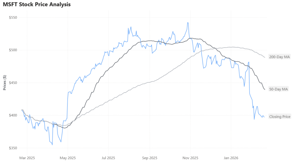
When we throw this measure into a line chart, along with our closing price, we can now start to see the 50-day trend which eliminates some of the noise of daily stock market volatility. And, if we wanted to see even longer trends, we can add a 200-Day moving average by manipulating our DAX measure.
If your base measure is a sum (i.e., Total Sales), then you would have to divide your rolling sum measure by the number of periods to get the average daily sales. For example, if you want the average daily sales over the last 30 days.
Rolling 30 Day Avg = DIVIDE ( [Rolling 30 Day Sales], 30 )This works well when:
- You truly want a fixed window of 30 days, and
- The data is fairly continuous (i.e., daily sales, daily bookings)
But this simple division can break down when dealing with:
- Missing days (no data on weekends, holidays, etc.)
- Non‑daily grains (i.e., monthly data)
At this point, you may already be thinking: “wait a minute… stock markets are closed on weekends, so our 50-Day and 200-Day moving average measures above will give inconsistent values”. And this would be the case if we were doing a sum and hard-coding our periods to be divided by.
For those cases, this is where the AVERAGEX pattern shines. Let’s check it out.
Step 4: Alternative Using AVERAGEX
The AVERAGEX pattern explicitly iterates over each date (or period) and averages the measure value. This avoids hard‑coding the days and plays nicer with missing days. Sticking with our Total Sales example above.
Rolling 30 Day Avg (Iterating) =
AVERAGEX (
    DATESINPERIOD (
        'Dates'[Date],
        MAX ( 'Dates'[Date] ),
        -29,              -- -29 gives you 30 days including the current day
        DAY
    ),
    [Total Sales]
)
Why -29 and not -30?
- DATESINPERIOD is inclusive of both ends
- A period of -29 days + the current day = 30 days total
What this does:
- Builds a table of dates (last 30 days).
- For each date, evaluates [Total Sales] in that daily context.
- Returns the average of those 30 values
This pattern is generally more semantically correct when you want “average per day over the last 30 days”.
4.1 Rolling 3-Month Average
If your visual is monthly (i.e., grouped by ‘Date'[Year & Month]), you may want a rolling 3‑month average. In that case, use months as the interval:
Rolling 3 Month Sales =
CALCULATE (
    [Total Sales],
    DATESINPERIOD (
        'Dates'[Date],
        MAX ( 'Dates'[Date] ),
        -3,
        MONTH
    )
)

Rolling 3 Month Avg = DIVIDE ( [Rolling 3 Month Sales], 3 )
Wrapping It Up...
Rolling averages (or moving averages) are a core DAX pattern every Power BI developer should know. They help with smoothing out noisy data, reveal meaningful trends, and enable better forecasting and decision-making discussions.
Just remember that before you get started with rolling averages (and other time-intelligence calculations), you’ll need a proper Dates table that is set up accordingly in your data model. Also, keep in mind the differences between forcing the periods (i.e., “30 days”) versus using the AVERAGEX function to deal with non-continuous data.
Need Help Getting Started With Power BI?
Our Microsoft Certified consultants can help with the implementation of Power BI in your organization